
| Recreational Mathematics Club | Discussion #4 |
| 12-Eye Portal Seed and the LLL algorithm
| |
| Speaker: Dhairya Baxi, Mahek Shamsukha | Indian Institute of Science |
A Linear Congruential Generator (LCG) is a simple pseudorandom number generator (PRNG) defined by the recurrence relation:
where the parameters are:
Each call to the generator updates the seed and outputs it (or some function of it) as the next pseudorandom value. The entire future sequence is thus fully determined by the initial seed and the triple (a,b,m).
The modular inverse of an integer a modulo m is the integer a−1 such that:

It exists if and only if gcd(a,m) = 1. When it does, it can be computed efficiently in O(log m) using the Extended Euclidean Algorithm:
Modular inverses let us “divide” in modular arithmetic, instead of computing x∕a mod m, we compute x ⋅ a−1 mod m.
We define two fundamental operations on an LCG state.
next(x) applies one step of the recurrence:

forward(x,n) applies next n times iteratively:
This runs in O(n) time, which is impractical for large n.
Unrolling the recurrence n times gives:

Applying the geometric series formula (for a≠1):

This reduces the problem to computing an mod m, which can be done in O(log n) via fast modular exponentiation.
 an ⋅ x + b ⋅ (an − 1) ⋅ inv_a1
 mod m
mod m
The modular inverse of (a − 1) exists whenever gcd(a − 1, m) = 1, which holds for typical LCG parameters.
Just as next applies the recurrence forward, prev(x) inverts it, recovering the state that would have produced x. Starting from:

we solve for xprev:

where a−1 is the modular inverse of a modulo m (which exists when gcd(a,m) = 1). In code:
 inv_a ⋅ (x − b)
 mod m
mod m
backward(x,n) applies prev n times, stepping the generator n steps into the past. The naive implementation runs in O(n):
Note that backward(x,n) is equivalent to forward(x,−n), so an efficient O(log n) version follows from the same closed form as before, substituting a−1 and −b ⋅ a−1 as the new multiplier and increment respectively.
The general problem is to find an initial seed whose LCG outputs fall within prescribed intervals over several consecutive steps. For a concrete application of this framework to finding Minecraft world seeds with fully-filled stronghold portals, see Appendix A.
More generally, the problem we study is:
Given bounds m1,M1,…,mk,Mk and an offset n, find an initial seed seed0 such that for each i ∈{1,…,k}:
That is, we want k consecutive outputs of the LCG, starting from step n, to each fall within a prescribed interval. The challenge is to search over the space of possible seeds seed0 ∈ [0,m) efficiently, brute force is infeasible when m is large (e.g. m = 248 in Java’s Random).
Using the closed form for forward, every constraint on seedn+i can be written directly in terms of seed0. Crucially, the offset n is handled for free: given any candidate seedn, we can recover seed0 = backward(seedn,n) in O(log n), or equivalently jump ahead with forward(seed0,n). This means we can freely translate between constraints on seed0 and constraints on any other step.
Expressing seedn+i = forward(seed0, n + i) via the closed form, the system of k constraints becomes (shown here for n = 0, k = 12):




Each constraint is a modular interval condition on seed0. The problem reduces to finding all seed0 ∈ [0,m) satisfying all k such constraints simultaneously.
The modular reduction is the main obstacle to solving the system directly. We eliminate it by observing that x mod m = x − km for some integer k ≥ 0. That is, for each constraint i there exists an unknown integer ki such that:
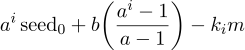
is the true (non-reduced) value. Substituting this into the bounds and rearranging, moving the b( )
term to both sides, each modular inequality becomes an ordinary linear inequality:
)
term to both sides, each modular inequality becomes an ordinary linear inequality:




The system now has k + 1 unknowns (seed0 and the integers k0,…,kk−1) and 2k linear inequalities over the integers. No modular arithmetic remains, the problem has been lifted to an integer linear feasibility problem.
We can write the system compactly by collecting the unknowns into a vector  = (seed0, k0, k1, …, kn−1)⊤
and defining:
= (seed0, k0, k1, …, kn−1)⊤
and defining:
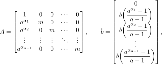
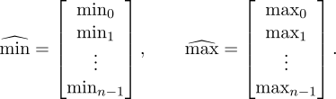
The entire seed-finding problem then reduces to finding an integer vector  such that:

subject to 0 ≤ x1 = seed0 < m. Crucially, the possible values of A +
+  mod m are exactly
the possible tuples of consecutive LCG seeds, so any solution
mod m are exactly
the possible tuples of consecutive LCG seeds, so any solution  directly yields a valid initial
seed.
directly yields a valid initial
seed.
The columns of A generate a lattice, the set of all integer linear combinations A for
for  ∈ ℤn. The
constraint
∈ ℤn. The
constraint  ≤ A
≤ A +
+  ≤
≤ asks for lattice points that land inside the axis-aligned box [
 ,
,  ]
after the shift by
]
after the shift by  .
.
Equivalently, applying A−1 to both sides transforms the axis-aligned box into a (potentially skewed)
parallelogram in the space of integer vectors  , and we seek all integer points inside that parallelogram.
This is illustrated below:
, and we seek all integer points inside that parallelogram.
This is illustrated below:

This reframing connects the seed-finding problem to classical problems in the geometry of numbers, and motivates the use of lattice reduction algorithms such as LLL to efficiently enumerate solutions.
Having reduced the problem to finding integer vectors  satisfying
  ≤ A
≤ A +
+  ≤
≤ , we now describe
how to enumerate all such solutions via branch and bound.
, we now describe
how to enumerate all such solutions via branch and bound.
Because A is lower triangular, the system  ≤ A
≤ A +
+  ≤
≤ can be solved one variable at a time from
the bottom row upward. Suppose components xi+1,…,xn−1 have already been fixed. Row i of the system
reads:
can be solved one variable at a time from
the bottom row upward. Suppose components xi+1,…,xn−1 have already been fixed. Row i of the system
reads:
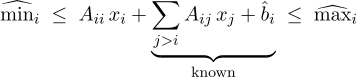
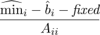
Isolating xi gives the real interval:

Since xi must be an integer, the feasible values are xi ∈{⌈li⌉,…,⌊ui⌋}. If ⌈li⌉ > ⌊ui⌋, the partial assignment is infeasible and the branch is immediately pruned.
The algorithm recurses from the last variable to the first, branching over all integer values in the feasible interval at each level:
 ,
,  ,
,  ,
,  , i)
, i) , bounds
  ,
,  ,
,  (components i+1,…,n−1 fixed), current index i
  satisfying
  ≤ A
≤ A +
+  ≤
≤

 full solution found
  , u ←
, u ←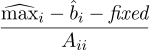
 prune: no valid integer exists
  ,
,  ,
,  ,
,  , i − 1)
 The outermost call is BranchAndBound(A,  ,
,  ,
,  , x, n− 1). Each leaf that reaches i < 0 yields a
valid
, x, n− 1). Each leaf that reaches i < 0 yields a
valid  , from which seed0 = x0 is read off directly.

The worst-case complexity is exponential in the number of solutions, but pruning makes it efficient in practice when the feasible parallelogram is small, which is precisely what LLL achieves by reducing the basis before running this search.
A lattice ℒ has infinitely many bases. If B = (b1,…,bn) is one basis and U is any unimodular matrix (integer matrix with detU = ±1), then BU is another valid basis generating the same lattice.
Observation. Two bases for the same lattice can produce parallelograms of wildly different shapes. A skewed basis yields a thin, elongated parallelogram; an orthogonal basis yields a compact, box-like one.
We want a basis B = (b1,…,bn) where:
Such a basis makes the corresponding parallelepiped well-shaped and better aligned with the coordinate axes, dramatically improving the performance of branch-and-bound methods.
Motivation for the next step. Finding an optimal basis (e.g. shortest or most orthogonal) is NP-hard in general. However, efficient approximation algorithms exist. The most celebrated is the LLL algorithm (Lenstra–Lenstra–Lovász, 1982), which computes, in polynomial time, a basis that is nearly orthogonal and well-balanced. In particular, it guarantees that the first basis vector is within an exponential factor of the shortest nonzero lattice vector.
Let B = (b1,…,bn) be a basis of a lattice ℒ⊂ ℝm. Let b1∗,…,bn∗ be its Gram–Schmidt orthogonalization:
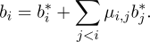
Definition 8.1. Let δ ∈ (1∕4,1). The basis B is called δ-LLL reduced if:
 ,
,

Theorem 8.2. If B is a δ-LLL reduced basis of ℒ, then

where λ1(ℒ) is the length of the shortest nonzero lattice vector.
Recall the Gram–Schmidt decomposition

where B∗ = (b1∗,…,bn∗) has orthogonal columns and M = (μi,j) is upper triangular with μi,i = 1.
Size reduction corresponds to modifying the columns of B using integer column operations so that

We proceed column by column. For j = 1,…,n, and for i = j − 1,j − 2,…,1, perform the operation

where ⌊⋅⌉ denotes rounding to the nearest integer.
This is an elementary column operation on B, and corresponds to updating the matrix M by

which ensures

Key point. Size reduction is achieved purely by integer column operations on B, preserving the lattice,
while ensuring all Gram–Schmidt coefficients satisfy |μi,j|≤ .
.
Theorem 8.3. Let B ∈ ℤm×n be an integer basis and let δ ∈ (1∕4,1). Then there exists an integer basis B′ such that:
Proof. We prove correctness and finiteness of the LLL algorithm.
(Correctness). If the algorithm terminates, then no Lovász condition is violated, and the basis is size-reduced. Hence the output basis is δ-LLL reduced.
(Lattice preservation). All operations used are integer column operations:
Thus the output basis is obtained from the input by unimodular transformations, and therefore generates the same lattice.
(Finiteness) Define a potential
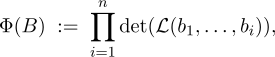
where ℒ(b1,…,bi) denotes the lattice generated by b1,…,bi.
Equivalently, since

we may write
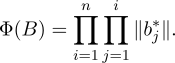
Effect of size reduction. Size reduction does not change the Gram–Schmidt vectors bj∗. Hence Φ(B) remains unchanged.
Effect of swapping bi,bi+1. All prefixes except the i-th remain unchanged, so only the factor

changes.
Let Φ′ denote the potential after swapping bi and bi+1.
First observe how the Gram–Schmidt vectors change. Consider the prefix

For this sequence, the Gram–Schmidt vectors are

where the first i − 1 vectors remain unchanged, and

Thus,

Now, since only the i-th prefix changes in the potential, we have

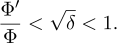
If the Lovász condition is violated, then

and hence

Taking square roots,
Finiteness. Observe that for each i,

where Bi is the matrix with columns b1,…,bi. Since Bi has integer entries, det(BiT Bi) is an integer, and hence each factor in Φ(B) is a square root of a positive integer.
Therefore, Φ(B) itself is a product of square roots of integers, and can take values only in a discrete subset of ℝ>0. In particular, in the interval (0,Φ(Bin)], it can assume only finitely many values.
Since each swap strictly decreases Φ(B) by at least a constant factor  < 1, the sequence of
potentials is strictly decreasing and cannot be infinite.
< 1, the sequence of
potentials is strictly decreasing and cannot be infinite.
Therefore, the algorithm terminates.
Combining the above, a δ-LLL reduced basis B′ exists. □
In Minecraft, an End Portal consists of 12 slots, each of which requires an Ender Eye to be filled. When a world is generated, each slot may already be pre-filled.
Internally, this is determined using calls to a pseudorandom generator (Random::nextFloat() in Java), which maps the internal seed to a value in [0,1). A slot is filled if this value exceeds 0.9.
The Java random number generator is a linear congruential generator:

In the world-generation pipeline, the first 760 calls are irrelevant for the portal. Thus, we begin at seed761 and require that the next 12 calls all satisfy

This translates to the constraint
![seedi ∈ [253327472328704, 248 − 1], i = 761,...,772,](index103x.svg)
since

Connection to our problem. This is an instance of the LCG constraint problem with:
Thus, finding a 12-eyed seed reduces to finding integer points satisfying linear constraints derived from an LCG, precisely the type of problem we studied using lattice methods and the LLL algorithm.

