Definition 1.2 (Constructive / basis definition). Let B = [b1,…,bk] ∈ ℝn×k have linearly independent columns. The lattice generated by B is

The matrix B is called a basis; n and k are the dimension and rank. When n = k the lattice is full rank.
| Recreational Mathematics Club | Discussion #2 |
| All about lattices
| |
| Speakers: Mahek Shamsukha, Dhairya Baxi | Indian Institute of Science |
Lattices are regular, discrete arrangements of points in Euclidean space. They arise naturally in crystallography, sphere packings, integer programming, cryptography, and coding theory. Two equivalent definitions are in common use.
Definition 1.1 (Algebraic definition). A lattice Λ ⊆ ℝn is a discrete additive subgroup of ℝn:
Definition 1.2 (Constructive / basis definition). Let B = [b1,…,bk] ∈ ℝn×k have linearly independent columns. The lattice generated by B is
The matrix B is called a basis; n and k are the dimension and rank. When n = k the lattice is full rank.
Key contrast with vector spaces. span(B) = {Bx : x ∈ ℝk} allows real coefficients and produces a continuous set. L(B) = {Bx : x ∈ ℤk} restricts to integer coefficients, producing a discrete set. Since the columns b1,…,bk are linearly independent, any y ∈ span(B) has a unique representation y = ∑ xibi, and y ∈ L(B) if and only if all xi ∈ ℤ.
Example 1.3. The standard integer lattice ℤn = {(x1,…,xn) : xi ∈ ℤ} is generated by the standard basis vectors of ℝn.
Example 1.4 (ℚn is not a lattice). The set ℚn is a subgroup of ℝn (it is closed under addition and subtraction), but it fails the discreteness condition. For any 𝜀 > 0, one can always find two distinct points x,y ∈ ℚn with ∥x − y∥ < 𝜀 (e.g. take x = 0 and y = (𝜀∕2,0,…,0)), so no uniform lower bound on pairwise distances exists. Hence ℚn is not a lattice.
A lattice can be represented by many different bases. Two bases B and C generate the same lattice if and only if B = CU for some unimodular matrix U.
Theorem 2.1. L(B) = L(C) if and only if there exists a unimodular matrix U (a square integer matrix with det(U) = ±1) such that B = CU.
Proof. (⇐) Suppose B = CU for some unimodular U. Since det(U) = ±1 and U has integer entries, U−1 is also an integer matrix, and

Hence every column of B is an integer combination of columns of C, giving L(B) ⊆ L(C), and symmetrically L(C) ⊆ L(B). Thus L(B) = L(C).
(⇒) Suppose L(B) = L(C). Since the columns of B lie in L(C), and vice versa, there exist integer matrices V,W such that

Substituting the second into the first,

Since the columns of B are linearly independent, we conclude V W = I. Taking determinants on both sides,

Since V,W have integer entries, det(V ),det(W) ∈ ℤ, so the only possibility is

Hence W is unimodular, and B = CW is the required relation with U = W. □
Given a lattice basis B = [b1,…,bn], it is often useful to transform it into an orthogonal system.
Definition 3.1. The Gram–Schmidt orthogonalization produces vectors B∗ = [b1∗,…,bn∗] defined iteratively by

In matrix notation, B = B∗M where M is upper triangular with 1s on the diagonal.
The vectors b1∗,…,bn∗ are mutually orthogonal and span the same vector space as B. However, the orthogonal vectors are usually not lattice vectors.
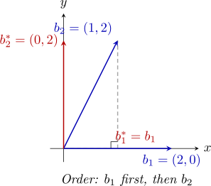
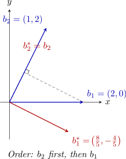
Example 3.2. Consider the basis B = {b1 = (2,0), b2 = (1,2)}. The two diagrams below show Gram–Schmidt applied in different orders.
Given a lattice basis B = [b1,…,bn], we define the fundamental parallelepiped

The translates 𝒫(B) + v for v ∈ L(B) partition all of ℝn; each coset of the lattice has exactly one representative in 𝒫(B).
Geometrically, det(L) measures the inverse density of lattice points: a large region of volume V contains roughly V∕det(L) lattice points. The determinant does not depend on the choice of basis.
Proposition 4.2. For any lattice basis B,

In particular, if B ∈ ℝn×n is square, then det(L(B)) = |det(B)|.
Proof. From the Gram–Schmidt factorisation B = B∗M, where M is upper triangular with 1s on the diagonal, we compute

Since M is upper triangular with 1s on the diagonal, det(M) = det(M⊤) = 1. Since the columns of B∗ are orthogonal, B∗⊤B∗ is diagonal with entries ∥bi∗∥2, so

Taking the square root,

Proof. Let v ∈ d ℤn be arbitrary, so v = dy for some y ∈ ℤn. We wish to find x ∈ ℤn such that

Recall the adjugate (classical adjoint) adj(B), whose (i,j) entry is the signed (j,i) cofactor of B. Since B ∈ ℤn×n, every cofactor is an integer determinant, so

The key identity relating the adjugate to the inverse is

Set x = adj(B)y. Since adj(B) and y are both integer, x ∈ ℤn. Moreover,

Hence v = Bx ∈ L(B), and since v was arbitrary, d ℤn ⊆ L(B). □
This shows that every integer lattice contains a scaled copy of the standard lattice as a sublattice.
This corresponds to the length of the shortest nonzero lattice vector. More generally, the successive
minima λ1 ≤ λ2 ≤ ≤ λn are defined so that λk(Λ) is the smallest r such that Λ contains k linearly
independent vectors of length at most r.
≤ λn are defined so that λk(Λ) is the smallest r such that Λ contains k linearly
independent vectors of length at most r.
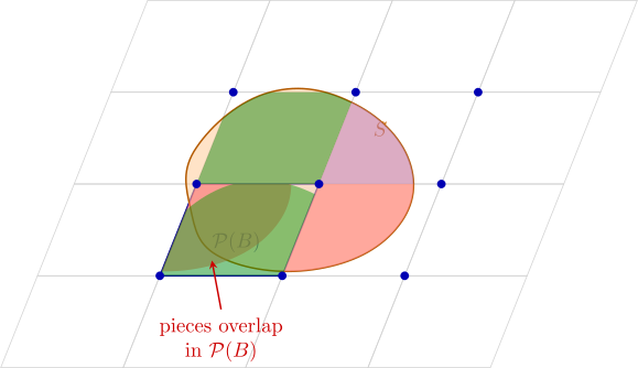
Blichfeldt’s theorem is essentially the pigeonhole principle for volumes: if a set S is too large to fit inside a single fundamental parallelepiped, then when we tile space with translates of 𝒫(B), at least two pieces of S must land in the same cell — and shifting them back reveals two points of S that differ by a lattice vector.
Theorem 6.1 (Blichfeldt). Let Λ = L(B) be a lattice and S ⊂ ℝn a measurable set. If vol(S) > det(Λ), then there exist two distinct points z1,z2 ∈ S such that z1 − z2 ∈ Λ.
Proof. Decompose S into the pieces that lie in each lattice-translate of 𝒫(B):

These sets are pairwise disjoint and cover S, so
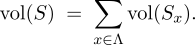
Now translate each piece back into 𝒫(B) by defining Tx = Sx − x ⊆𝒫(B). Since translation preserves volume,

Since all Tx live inside 𝒫(B) and their total volume exceeds vol(𝒫(B)), they cannot all be disjoint. Hence there exist distinct x≠y ∈ Λ such that Tx∩Ty≠∅. Pick any point p in this intersection. Then

and

The diagram below illustrates the idea in ℝ2: a blob S is cut by the lattice tiling, each piece is translated into 𝒫(B), and two pieces overlap.
Theorem 7.1 (Minkowski). Let Λ be a lattice in ℝn and let S be a convex, centrally symmetric body. If

then S contains a nonzero lattice point.
Proof. Apply Blichfeldt to S∕2 = {x : 2x ∈ S}, which satisfies vol(S∕2) = 2−n vol(S) > det(Λ). Blichfeldt gives distinct z1,z2 ∈ S∕2 with z1 − z2 ∈ Λ ∖{0}. Then 2z1,2z2 ∈ S, so by symmetry −2z2 ∈ S, and by convexity

This theorem gives an upper bound on the shortest lattice vector:

Idea of the proof. Since p ≡ 1 (mod 4), there exists i such that i2 ≡−1 (mod p).
Consider the lattice generated by
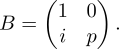
By Minkowski’s theorem, there exists a nonzero lattice vector (a,b)⊤ satisfying 0 < a2+b2 < 2p. Using i2 ≡−1 (mod p), one checks that p∣a2 + b2. Since the value lies strictly between 0 and 2p, we must have a2 + b2 = p. □
The Hermite Normal Form (HNF) provides a canonical, unique representation for a lattice. We say a matrix B = [b1,…,bn] of full row rank is in HNF if it has the form B = [H∣0], where:
Definition 9.1. A square matrix H = [hij] is in Hermite Normal Form if:
In particular, H is nonsingular. The HNF is computed by applying elementary column operations, which are special unimodular transformations:
Since these are unimodular, they preserve the lattice generated by the columns of B.
Theorem 9.2 (Existence of HNF). Every rational matrix of full row rank can be brought into Hermite normal form by a sequence of elementary column operations. Equivalently, for every such matrix B there is a unimodular matrix U such that BU is in HNF.
Proof. Without loss of generality assume B is integral (otherwise clear denominators). We build a sequence of matrices
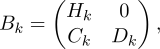
where Hk is a k×k matrix already in HNF. At each step, let d1,…,dn−k be the first-row entries of Dk. By permuting columns and negating, assume all di ≥ 0 with at least one nonzero. If two nonzero entries di > dj appear, add −⌊di∕dj⌋ times column j to column i, strictly reducing the total sum of first-row entries. Repeating (this executes the Euclidean algorithm on pairs of entries) terminates with a single nonzero entry d in the first row of Dk, which is placed in the first column by a swap. Finally, for each i = 1,…,k, subtract ⌊ci∕d⌋ times the new column from column i to reduce all entries in the first row of Ck to the range [0,d). This yields Bk+1 with Hk+1 of size (k + 1) × (k + 1) in HNF. □
Remark 9.3. The naive algorithm above may be non-polynomial due to intermediate entry growth. A polynomial-time variant exists by performing all arithmetic modulo the determinant of the relevant submatrix, keeping entries bounded throughout.
Let Λ′ = L(B′) be a sublattice of Λ = L(B), both full-dimensional. Then B′ = BV for some integral matrix V , and the index of Λ′ in Λ is

Proof. Let B,B′ be bases of Λ,Λ′ with B′ = BV and D = |det(V )|. Then B = B′V −1 and DV −1 is an integral matrix (since the entries of V −1 = adj(V )∕det(V ) become integral upon multiplication by D). Hence

so DΛ ⊆ Λ′. □
Theorem 9.5 (Bases in HNF). Let Λ′ be a sublattice of Λ.
Using HNF and the dual lattice, the following problems are all solvable in polynomial time: computing a basis for L(B), deciding whether L(B) = L(C), membership testing (v ∈ L(B)?), union, and containment.
In contrast, the following are believed to be computationally hard.
Definition 10.1. The Shortest Vector Problem (SVP): given a lattice basis B, find a nonzero lattice vector of length at most γ ⋅ λ1(L(B)).
Definition 10.2. The Shortest Independent Vectors Problem (SIVP): given a rank-n basis B, find n linearly independent lattice vectors of length at most γ ⋅ λn(L(B)).
Definition 10.3. The Closest Vector Problem (CVP): given a basis B and a target vector t, find a lattice vector within distance γ ⋅ dist(t,L(B)).
These notes follow the exposition in:



