Recreational Mathematics Club


Recreational Mathematics Club	Discussion #1

Introduction to Ehrhart Theory

Speaker: Dhairya Baxi	Indian Institute of Science

1 Introduction and Motivation

How many integer-coordinate points fit inside a triangle drawn on grid paper? Inside a square of side length t? Inside an arbitrary convex shape whose vertices lie on a lattice? These questions sit at the crossroads of combinatorics, geometry, and algebra, and they admit surprisingly clean answers.

Definition 1.1. A lattice polytope (or integral polytope) P ⊂ ℝ^d is a convex polytope whose vertices all lie in ℤ^d. Its lattice-point count is

( ) LP(t) := # tP ∩ ℤd , t ∈ ℤ >0,

where tP = {tx : x ∈ P} is the t-th dilate of P.

Our main goal is to understand why L_P(t) turns out to be a polynomial in t. Along the way we will encounter:

Pick’s theorem — an exact formula in the plane,
Reeve tetrahedra — a cautionary tale showing Pick’s theorem does not generalise naïvely to 3-D,
Integer-point transforms — a generating-function toolkit,
Brion’s theorem — a beautiful identity decomposing a polytope via its vertex cones,
Ehrhart’s theorem — the punchline: L_P(t) is always a polynomial.

2 Pick’s Theorem

2.1 Statement

Theorem 2.1 (Pick, 1899). Let P ⊂ ℝ² be a lattice polygon (a 2-dimensional lattice polytope). Denote by

I = number of interior lattice points of P, B = number of boundary lattice points of P.

Then

|----------------------| |Area(P ) = I + B-− 1.| -----------------2-----

2.2 Example

Example 2.2. Consider the lattice polygon with vertices (0,0), (4,0), (1,3). One counts B = 4 boundary lattice points and I = 3 interior lattice points. Pick’s theorem gives

Area = 3+ 42 − 1 = 4.

(Verify directly: area = 1
2 |4 ⋅ 3 − 0| = 6. Hmm — recount: the vertices (0,0),(4,0),(1,3) give area det (4 1)

0 3 = 6. Here B = 5, I = 3: 3+5∕2−1 = 4.5≠6. Recount boundary points carefully as an exercise!)

Figure 1: A lattice polygon illustrating Pick’s theorem.

2.3 Connection to the Ehrhart polynomial

For a lattice polygon P with area A, boundary count B, and interior count I, the Ehrhart polynomial is

2 B- LP (t) = A t + 2 t+ 1.

Comparing with Pick’s theorem (A = I + B∕2 − 1) recovers the classical formula as the special case t = 1.

3 Reeve Tetrahedra: Pick’s Theorem Fails in 3-D

3.1 The construction

Definition 3.1. For a positive integer r, the Reeve tetrahedron T_r is the lattice tetrahedron with vertices

v0 = (0,0,0), v1 = (1,0,0), v2 = (0,1,0), v3 = (1,1,r).

Figure 2: The Reeve tetrahedron T_r. Despite growing volume vol(T_r) = r∕6, the lattice-point data (I = 0,B = 4) is independent of r.

3.2 Why this is a counterexample

Proposition 3.2. For every r ≥ 1:

(i): T_r has no interior lattice points: I(T_r) = 0.
(ii): T_r has exactly 4 boundary lattice points (its four vertices): B(T_r) = 4.
(iii): vol(T_r) = r∕6.

Proof sketch. The four faces of T_r are lattice triangles. One verifies (e.g. by checking the relevant determinants or using the characterisation of integer points as solutions to integer linear systems) that each face contains no lattice points beyond its vertices, and that the interior is likewise empty. The volume formula follows from vol(T_r) = 1
6 |det[v₁−v₀, v₂−v₀, v₃−v₀]| = 1
6 |det ( )
1 0 0
( 0 1 0)
1 1 r | = r∕6. □

Moral. The family {T_r}_r≥1 shows that in 3-D (and higher), the lattice-point data (I,B) alone does not determine the volume. Any naive 3-D analogue “vol(P) = aI + bB + c” would have to satisfy r∕6 = c for all r, which is impossible. Pick’s theorem has no direct analogue in dimension ≥ 3.

3.3 What replaces it?

The right framework is the Ehrhart polynomial, which we derive in Sections 4–6. For the Reeve tetrahedra,

L (t) = rt3 + t2 + 6−--rt+ 1, Tr 6 6

so the volume appears as the leading coefficient rather than as a simple linear combination of I and B.

4 Integer-Point Transforms for Rational Cones

4.1 Motivation: encoding lattice points as generating functions

Instead of merely counting lattice points, we list them inside a single algebraic object.

Definition 4.1. Let S ⊂ ℝ^d. The integer-point transform of S is the formal sum of Laurent monomials

∑ ∑ σS(z) := zm = zm1zm2 ⋅⋅⋅zmd. d d 1 2 d m ∈S∩ℤ m∈S∩ ℤ

Setting z = 1 (all z_i = 1) recovers the lattice-point count: σ_S(1) = #(S ∩ ℤ^d).

4.2 Warm-up: the ray

Example 4.2. The 1-dimensional cone K = [0,∞) gives the familiar geometric series:

∑ 1 σK (z) = zm = -----. m ≥0 1− z

4.3 A 2-dimensional cone and the fundamental parallelogram

Example 4.3 (cf. Example 3.4 in the reference). Let

K := {λ1(1,1)+ λ2 (− 2,3) : λ1,λ2 ≥ 0 } ⊂ ℝ2.

Define the fundamental parallelogram

Π := {λ1(1,1)+ λ2(− 2,3) : 0 ≤ λ1,λ2 < 1}.

We tile K by translating Π by all nonnegative integer linear combinations of (1,1) and (−2,3). The integer points in Π are

2 Π ∩ ℤ = {(0,0 ),(0,1),(0,2),(− 1,2),(− 1,3)}.

Therefore:

1+ z2 + z2+ z− 1z2 + z−1z3 σK (z) = ---------2---1--2−2-31--2. (1− z1z2)(1 − z1 z2)

Figure 3: The 2-D cone K and its fundamental parallelogram Π (cf. Figure 3.5 of the reference).

4.4 The main theorem for simplicial cones

Definition 4.4. A simplicial d-cone is a cone of the form

K = {λ1w1 + ⋅⋅⋅+ λdwd : λ1,...,λd ≥ 0}

where w₁,…,w_d ∈ ℤ^d are linearly independent. The fundamental parallelepiped is

Π := {λ1w1 + ⋅⋅⋅+ λdwd : 0 ≤ λ1, ...,λd < 1}.

Theorem 4.5 (Integer-point transform of a simplicial cone). Let K = {λ₁w₁ + ⋅⋅⋅ +λ_dw_d : λ_k ≥ 0} be a simplicial d-cone with w_k ∈ ℤ^d, and let v ∈ ℝ^d. Then

σv+K (z) = ----------σv+-Π(z)----------, (1− zw1 )(1 − zw2)⋅⋅⋅(1− zwd)

where Π is the fundamental parallelepiped of K.

Proof idea. Every lattice point m ∈ (v + K) ∩ ℤ^d can be uniquely written as

m = p + k1w1 + k2w2 + ⋅⋅⋅ + kdwd,

with p ∈ (v + Π) ∩ ℤ^d and k₁,…,k_d ∈ ℤ_≥0. This is the decomposition λ_j = ⌊λ_j⌋ + {λ_j} applied to each coefficient. Expanding the right-hand side of the claimed identity as a product of geometric series yields exactly this decomposition. □

Key geometric idea. We tile the cone v + K with translates of the parallelepiped v + Π. The denominator (1 −z^w₁) ⋅⋅⋅ (1 −z^w_d)⁻¹ accounts for all nonnegative integer translates; the numerator σ_v+Π accounts for the “starting points” inside Π.

Corollary 4.6. For any pointed rational cone K, the integer-point transform σ_K is a rational function of z.

5 Brion’s Theorem

5.1 A surprising 1-D warm-up

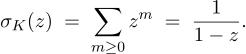
Suppose we want to list all positive integers via a generating function:

2 3 ∑ k --x-- x + x + x + ⋅⋅⋅ = x = 1 − x. k>0

(1)

Similarly, we can list all integers up to 5:

⋅⋅⋅+ x −1 + x0 + x1 + ⋅⋅⋅+ x5 = ∑ xk = --x5---. 1− x−1 k≤5

(2)

Adding the two rational functions gives a miraculous cancellation:

x x5 x x6 x − x6 ----- + -----−1 = ----- + ----- = ------ = x+ x2 + x3 + x4 + x5. 1 − x 1− x 1 − x x − 1 1− x

(3)

The sum of two rational functions, each representing an infinite series, collapses to a polynomial representing the finite set {1,2,3,4,5}.

Geometrically: (1) is the integer-point transform of the ray [1,∞) (the vertex cone at the left endpoint of the interval [1,5]), and (2) is the integer-point transform of the ray (−∞,5] (the vertex cone at the right endpoint). Their sum encodes the integer points in the interval [1,5]. This is Brion’s theorem in dimension 1.

Figure 4: Brion’s theorem in 1-D: two infinite vertex-cone series cancel to the finite interval series (cf. Beck–Haase–Sottile §1).

5.2 A 2-D example: the quadrilateral

Let Q be the quadrilateral with vertices (0,0), (2,0), (4,2), (0,2). At each vertex v we form the vertex cone K_v: the cone with apex v generated by the two edge directions leaving v. By Theorem 4.5, each vertex cone has a rational integer-point transform:


Vertex v	Cone K_v	σ_{K_v}(x,y)

(0,0)	ℝ_≥0(1,0) + ℝ_≥0(0,1)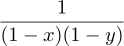

(0,2)	(0,2) + ℝ_≥0(0,−1) + ℝ_≥0(1,0)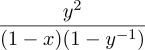

(4,2)	(4,2) + ℝ_≥0(−1,0) + ℝ_≥0(−1,−1)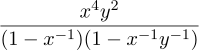

(2,0)	(2,0) + ℝ_≥0(1,1) + ℝ_≥0(−1,0)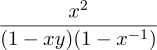

Summing these four rational functions:

	+ + +
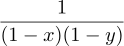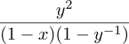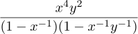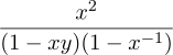	= y² + xy² + x²y² + x³y² + x⁴y² + y + xy + x²y + x³y + 1 + x + x²,

which is exactly the polynomial listing the 12 integer points of Q. The four infinite rational functions collapse, pole-free, to a finite polynomial.

Figure 5: The quadrilateral Q and its four vertex cones. Summing the vertex-cone generating functions gives the lattice-point polynomial of Q.

5.3 Statement of Brion’s theorem

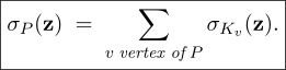
Definition 5.1. Let P ⊂ ℝ^d be a polytope and v a vertex of P. The vertex cone (or tangent cone) of P at v is

Kv := v + cone{u− v : u ∈ P },

the smallest cone with apex v that contains P. Its integer-point transform σ_{K_v}(z) is a rational function by Corollary 4.5.

Theorem 5.2 (Brion, 1988). Let P ⊂ ℝ^d be a rational polytope. Then, as rational functions,

|--------------------------| |σ (z) = ∑ σ (z).| | P Kv | ----------v vertex ofP------

Why this is remarkable. Each σ_{K_v} is a rational function with poles at z = 1; the vertex cones are unbounded and their lattice points vastly overlap. Yet summing over all vertices, every pole cancels and every overlap cancels, leaving the polynomial σ_P — finite because P is bounded. As Beck, Haase, and Sottile write, the formula “provokes a slight feeling of mystery” even after years of study.

5.4 Why Brion’s theorem is useful

Brion’s theorem converts a problem about the bounded polytope P into a sum of problems about cones, for which Theorem 4.5 provides explicit rational-function formulas. It is the key bridge between the geometry of polytopes and the algebraic machinery of generating functions.

Concretely, to compute L_P(t) = #(tP ∩ ℤ^d):

1.: Triangulate each vertex cone into simplicial cones.
2.: Use Theorem 4.5 to write each simplicial cone’s integer-point transform as an explicit rational function.
3.: Apply Brion’s theorem to sum over all vertices.
4.: Read off the Ehrhart polynomial from the resulting expression.

6 Ehrhart’s Theorem

6.1 The Ehrhart series

Definition 6.1. The Ehrhart series of a lattice polytope P is the generating function

∑ t EhrP (z) := 1 + LP (t) z. t≥1

The key observation is that the Ehrhart series can be recovered from the integer-point transform of the cone over P.

Definition 6.2. Given a lattice polytope P ⊂ ℝ^d with vertices v₁,…,v_n, lift each vertex to ℝ^d+1 by setting w_j = (v_j,1). The cone over P is

cone(P ) := {λ1w1 + ⋅⋅⋅+ λnwn : λj ≥ 0} ⊂ ℝd+1.

The dilate tP is recovered by slicing cone(P) with the hyperplane x_d+1 = t.

Figure 6: Recovering dilates of P inside cone(P) (cf. Figure 3.6 of the reference).

Lemma 6.3. σ_cone(P)(1,1,…,1,z) = Ehr_P(z).

Proof. The terms with z_d+1^t in σ_cone(P) correspond to lattice points in the slice x_d+1 = t, which is exactly tP ∩ ℤ^d. Summing gives Ehr_P(z). □

6.2 The main theorem

Theorem 6.4 (Ehrhart, 1962). If P is an integral convex d-polytope, then L_P(t) is a polynomial in t of degree d.

Proof (following the reference). By triangulating P into integral simplices (using no new vertices), it suffices to prove the result for a single integral d-simplex Δ.

Let Δ have vertices v₁,…,v_d+1 ∈ ℤ^d, and set w_j = (v_j,1) ∈ ℤ^d+1. Then cone(Δ) is a simplicial (d + 1)-cone. By Theorem 4.5,

--------σΠ(z)--------- σcone(Δ)(z) = (1− zw1)⋅⋅⋅(1 − zwd+1),

where Π = {∑ _jλ_jw_j : 0 ≤ λ_j < 1}.

Specialising z₁ = ⋅⋅⋅ = z_d = 1 (so z^w_k → z_d+1¹) and applying Lemma 6.3:

Ehr (z) = ---g(z)---, Δ (1 − z)d+1

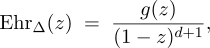
where g(z) = σ_Π(1,…,1,z) is a polynomial of degree ≤ d (since every point in Π has last coordinate < d + 1, hence ≤ d). Moreover g(1) = #(Π ∩ ℤ^d+1) ≥ 1 (the origin lies in Π), so g(1)≠0.

By the following standard lemma, this implies L_Δ(t) is a polynomial of degree d. □

Lemma 6.5. If ∑ _t≥0f(t)z^t = g(z)∕(1 − z)^d+1 where g is a polynomial, then f is a polynomial of degree d if and only if deg(g) ≤ d and g(1)≠0.

7 Summary and Further Directions

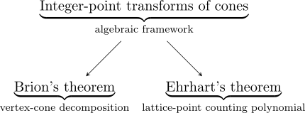
Here is the logical thread we have followed:

Pick’s theorem f−−ai−ls i−n− 3−-−D→ Reeve tetrahedra r−−ig−ht− f−ra−m−e−w−o−r→k LP(t) ◟-----◝◜-----◞ ◟------◝◜------◞ ◟ ◝◜-◞ dim 2, exact counterexample polynomial

IntBergiEeohrnr- pho’sairnthtte’ostr trehamenosrfoermms of cones
◟-◟-◟----◝◜◝◜--◝◜◞---◞---------◞
vlearttteicxe- c- pooniaentl dgeecobcourmnaipticon fsgrait pmiooenlywnoormkial

Some avenues for further exploration:

Rational polytopes. If the vertices of P are in ℚ^d (not necessarily ℤ^d), then L_P(t) becomes a quasi-polynomial — periodic coefficients instead of constant ones.
Barvinok’s algorithm. An efficient (polynomial-time in fixed dimension) algorithm to compute L_P(t), based on signed decompositions of cones and Theorem 4.5.
h^∗-vectors and unimodality. The h^∗-polynomial of a lattice polytope is conjectured to be unimodal in many settings; this remains open in general.
Connections to commutative algebra. The Hilbert series of a graded ring associated to P equals Ehr_P(z), linking Ehrhart theory to algebraic geometry.
Mixed volumes and the BKK theorem. Counting solutions of sparse polynomial systems leads naturally to mixed Ehrhart theory.

Acknowledgements

These notes follow closely the exposition in:

M. Beck and S. Robins, Computing the Continuous Discretely, 2nd ed., Springer, 2015 (Chapter 3).
M. Beck, C. Haase, F. Sottile, Formulas of Brion, Lawrence, and Varchenko on Rational Generating Functions for Cones

Some images taken from Wikipedia